Multivariate forecasts

Multivariate projection models are different to univariate in that the solution to the model, which ultimately forms the basis of the projection of the future, is interdependent on other variables in the model. Thus, before we can project say the level of interest rates, we need to know the level of inflation, while at the same time, before we can project the level of inflation, we need the know the level of interest rates.
Such interdependencies often requires that the system or model be solved iteratively: we basically pick a random level for inflation and use that to solve for the interest rate. Then we use that interest rate to solve for inflation, and continue in this fashion, until the solution converges to a stable answer, which it usually does.
One example of such an interdependent model is the Ferra Econometric Model or FEM, which is also discussed here.
Core and satellite approach
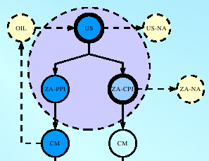
FEM is developed in a core and satellite approach, the order of the satellites dictated by the causal relationships between variables and groups of variables. Thus the first satellite, for example, is used to model the US economy, the next satellite for the Japanese economy and only then the third satellite is used to model the SA economy. Events in the US will impact Japan and South Africa and events in Japan will impact in South Africa. Using the combination of the US and Japanese economies as a proxy for the world economy, world economic events thus flow through to South Africa and together these three economies form the economic core of the FEM model.
Since satellites can be easily added or removed, the FEM economic core is often reduced to the US and SA satellites, as shown in the snapshot given above.
Dynamic response
In the development of the FEM model, a considerable amount of effort is spent on ensuring that the dynamic responses of the model are sound. A predefined set of impulses are played through the model and the model's responses to these are calculated, both in absolute terms and as deviations from a clean simulation. These responses are inspected and equations are adjusted in order to ensure a proper working of the model. The responses also provide quality information from a policy or risk management perspective.
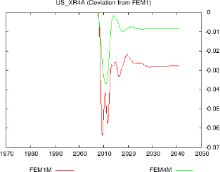
The response shown above displays a combination of the quarterly and annual FEM response, here of the real effective US exchange rate to an increase in the real US money supply. The overshoot shown corresponds to theory and is very similar between the two models. The quarterly and annual models are always played off against one another and provides an import additional check for model consistency. In the longer term, the annual model's response will dominate, which is encouraging, as the theoretical response should be a 1% drop. Note how close the estimated, uncalibrated equation approximates theory.
Amalgamation of models and horizons
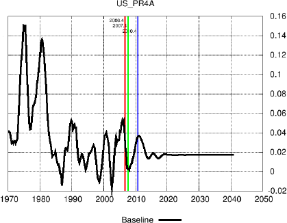
At present, FEM models three different horizons: monthly, quarterly and annually. This helps with the short and long term accuracy of the model, as these aspects are treated separately but combined in FEM. It also cuts back dramatically on the calibration of the model via add factors, as the way in which the models are integrated ensures a smooth transition from actuals to projections, and from horizon to horizon.
Note in the projection above, of US producer inflation, how the baseline moves from the actual to the monthly, univariate projection models' output (beyond the red line) and then to the quarterly econometric (beyond the green line) and finally to the annual model (beyond the blue line) and then how it settles on the long term equilibrium level, encouragingly close to the in-sample average of the series.
Projections
FEM is used to prepare a number of projections. Note how South Africa's economic growth rate is projected to remain high until after 2010, when the soccer world cup is scheduled to be held in the country. Even beyond this date, given the correct policy mix, a growth rate of 4% per year is sustainable.
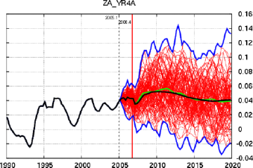
Risk
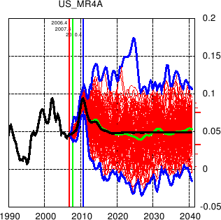
The example given here shows the growth in US money supply. After an initial period of rapid acceleration, this reverts back to the long run steady state growth rate of more or less 5% yoy. Note the distribution that is shown on the right hand axis and that is obtained via a Monte Carlo type simulation of the model. The simulation smoothly transits from the monthly to the quarterly to the annual model, shock effects from the one carried forward into the next until it has worked itself out of the system.
These type of simulation results are often used as input into subsequent models, such as valuation models, and used to construct various risk measures, such as cost at risk (CAR) or economic risk type measures.